Home » 2013
Yearly Archives: 2013
Review of Udacity CS101
One of the main reasons that I’ve been neglecting writing articles is that I had been taking the CS101 Udacity course. Udacity is a MOOC, short for massive open online course. That means that anyone can go online to register and take the course. Most MOOCs, including Udacity are usually free. I am a huge fan of MOOCs and this is the second course that I’ve finished. The first was on Coursera (Introduction to Computational Finance and Financial Econometrics — recommended). Although there are ways to get “credit” for taking a MOOC, my goals have been personal/professional development.
CS101 can be found here. Udacity divides their course catalog into Beginner, Intermediate and Advanced categories. CS101 is listed as a beginner course. CS101 teaches an introduction to Computer Science (CS). The class uses Python as its programming language for examples and assignments. To provide students with a coherent project that illustrates various aspects of CS, the class builds a simple search engine.
This happened to fit my needs quite well. I wanted a platform that could do the work of R but also provide a better framework for putting together small programs that I could use to automate tasks. I am also interested in Quantopian and their Zipline backtesting engine. It is written in Python and it might facilitate my research in short term trading strategies. Finally, I have an idea for an internet security & privacy product. Learning about search engines seemed terrific background. And the price was right: free.
My background includes a degree in computer engineering and I’ve done some coding professionally. I am not a beginner nor am I a current professional. I looked forward to a review of CS fundamentals.
CS 101
David Evans teaches the course. The course description indicates “no prior programming knowledge needed.” Although perhaps not needed, I’d recommend some prior programming. It need not be extensive but it would be extremely helpful to have done some coding, some thinking about coding and made some mistakes. Udacity recently added another, more basic course, “Intro to Programming in Java” that I believe was added because of similar feedback. My recommendation for the target audience is someone already coding at the beginner or intermediate level that is looking to add some formality to their effort. Unlike the CS101 course that I took in school, there are no proofs in this class (if you don’t know what I’m referring to, don’t worry).
The course is made up of 11 sections presumably corresponding to week per section. The original course had 7 sections but was subsequently extended. Each lesson is made up of a video lecture, quizzes and problem sets. Professor Evans comes across in a friendly, somewhat purposefully nerdy manner that worked. A key part of the success of the course is the many quizzes and exercises. The quizzes are interspersed inside the lectures and need to be answered, though not correctly, to move on. Professor Evans goes over the answer with an explanation. Properly used, these quizzes keep students’ minds engaged and active rather than passive.
The problem sets come after the lecture. Problem sets include multiple choice questions and/or coding assignments. The course allows for the user to code in an online Python editor that enables a student to avoid having to go through a local Python installation. This takes the sometimes painful step of installation away from the process. There is a computerized grading mechanism for student code. It worked but sometimes could be tricked. I don’t feel this is a terrible shortcoming as my take is that most or all of the students are enrolled for their own benefit. Hence, any “cheating” truly is only cheating yourself. The coding assignments did not involve much typing but instead usually demanded thinking computer science-ly. This is where I felt that having some coding experience helps. This type of thinking involves looking at the world differently and requires a bit of practice.
In addition to the course itself, there is a discussion section where students can post questions, comments or offer help. Frankly, I did not take much advantage of this. Other students would post code that they thought did the job particularly well or cleverly, to figure out what was wrong with their code or even where to begin thinking about something. My recollection is that answers appeared quickly; so there is help available when one gets stuck. Plus, all problem sets have included video answers. It is worth noting that Professor Evans and the other instructors do respond in the forums.
What makes this course particularly good is that it is not teaching a programming language but does teach Computer Science. This is not the same as teaching a programming language although CS is about programming but in a more global, holistic way. The difference may seem small but a reasonable analogy would be the skill of say, steel-working vs. civil engineering. If you are going to design and build a bridge, it will involve a theory of what keeps bridges from falling (the theory or CS) and the actual building of the steel framework (programming). A good designer will understand the programming and be able to choose the correct tools for the job, i.e., the best environment and programming language. But the design or algorithm, should transcend the particular tool. In fact, computer scientists create programming languages for particular (or general) problem types.
Many quizzes involve what appear to be trick questions. These are not meant to be tricky but to point out how some of the details of the Python interpreter influence code behavior. It provides examples for how to think about debugging programs and the types of things that can go wrong. It would be helpful had the course explicitly noted that other programming languages handle things slightly differently and therefore it is useful to understand the details. Ultimately a programmer will find out the details, it is just a question of find out the easy way or the hard way. One section that is very helpful to beginners was the section that covered how to learn new techniques and/or libraries.
Professor Evans gives the three main themes of Computer Science: abstraction, universality and recursion. My CS professor from school would add that CS is about managing complexity. These are discussed in terms of solving actual problems and that makes it extremely relevant to the student. And I think it is important to rise above the details of programming and get an idea of how to think about problems using data structures and algorithms. This manner of thinking is beneficial beyond computer science – it has served me well in thinking about economics and finance.
Conclusion
The stated goal is that the student will “have learned key concepts in computer science and enough programming to be able to write Python programs.” The course does an excellent job of doing this. As I stated before, I recommend at least some coding experience. The video lectures, with the support of the discussion forums, provide a clear exposition of the material in an easy-going manner. Professor Evans covers the key concepts for an introduction to computer science and to the fundamental tools to get programming jobs done. The quizzes and problem sets are what bind the whole experience together. Watching lectures alone cannot teach; learning is about doing. There is plenty of both to be had in Udacity’s CS101 class.
Brinkmanship Provided Opportunities in T-Bills
Last week, just prior to the temporary resolution of the debt ceiling issue, I wrote up this article for Seeking Alpha. It covered two topics. The first was about a couple of articles discussing price action in the Bill markets. The second and more interesting part illustrated how investor preferences were creating arbitrage opportunities for T-Bill investors. Let me know what you think.
To (QE-)Infinity and Beyond
Please check out my new article at Seeking Alpha. It discusses Fed QE exit strategies and what could go right or wrong.
Book Review: Volatility Trading
This is a book about trading volatility professionally. The target audience is those who already have some familiarity with options theory and are ready to use math in their market analysis. One does not need to be a professional options trader but the book instructs a professional attitude toward trading.
It accomplishes two goals very well. First, it delivers a set of knowledge about volatility markets. Second, it delivers the message that trading is hard and demands deliberate focus. So while the actual material is on the volatility markets, the theme of the book is that one should use all of tools at our disposal, use a systematic methodology and target continuous improvement. In short, if you wish to learn about volatility trading or, in general, how to approach trading of any sort as a business, you will benefit greatly from Volatility Trading. This is not idle talk. I ran an options trading desk and purchased a copy for each person working for me.
Despite having a PhD (yes, despite) and including the relevant math, Sinclair is clear and overwhelmingly practical. Even for those that already trade volatility products, as I do, there is much value in the material. He does much work for us, including:
1) Reading a vast amount of academic and industry research, as well as conducting his own; then highlighting the most valuable nuggets.
2) He puts into clear prose and practical context those most valuable results. For example, the explanation of why leveraged ETF’s erode in value but are not “destined to go to zero” was illustrated nicely with text that complemented the math. Math is necessary and adds to the explanation.
3) He puts the theory into the context of practical reality. Although this is most obvious when he discusses the shortcomings but utility of the Black-Scholes framework, it comes through elsewhere such as under what circumstances higher efficiency estimators fail back into the daily close-close estimator.
That said, there is subject matter relevant to volatility trading that is not covered but still important to volatility trading. For example, volatility options (VIX options) or dealing with portfolios of options. The subjects covered are, for the most part, covered well – the section on behavioral finance is, understandably, given only a quick run through. Even in this section, the practical nature of Sinclair’s outlook shows through as he discusses that we should mind our own foibles for mistakes but also look to those same foibles for sources of potential edge.
From the perspective of trading as a professional, Sinclair bangs the drum on:
1) Quantify what you can.
2) Remember #1, but using non-quantifiable information is valuable and, often, necessary.
3) Understanding that trading, particularly options trading that is so path dependent, is about playing the probabilities. Keep the long run in mind.
4) Trading requires having an edge; to best exploit it, understand it and the tools you use.
5) Emphasize the practical, particularly developing a process.
I cannot provide a review of the web site as I have not yet used it.
I will conclude with Sinclair’s own words: “Successful trading is about developing a consistent process.” Knowledge is essential but insufficient. I think that is what Euan Sinclair would hope the reader came away with and kept. Everything else can be researched – and much of it can be found in “Volatility Trading.” I find it very valuable and highly recommend it.
If you enter Amazon through my site (the image above), I will get a small commission. I am experimenting with this as a source of revenue for my blog. Hopefully reviewing the book (and my other posts) added some value. If so, great. Incidentally, the commission is already built into Amazon prices and the price stays the same whether you enter from my site or not.
We Interrupt Our Regularly Scheduled Programming
I was doing my morning reading prior to the release of NFP, and came across this article from Bloomberg. The article is about Takeshi Fujimaki. In addition to being a “former adviser” to George Soros, he won a seat in Japan’s upper house of parliament last month. He calls the JGB market a bubble which has been said before but the very last paragraph blew me away:
“It’s impossible to avoid a default at this point, but what’s important is to create a system to avoid the same mistake and that’s where I can contribute as a politician,” Fujimaki said.
By the way, I found the above paragraph even more staggering than the one before it. In the paragraph before, Fujimaki said that “The yen’s fundamentals suggest to me it should be around 180 to 200 per dollar.”
Wow. We have all read (and re-read) Kyle Bass on how Japan is about to implode (I’ll add that I am a fan of Bass). There is a massive difference, however, between a hedge fund manager suggesting JGB’s collapse and an elected politician (even if ex-hedge fund) comes out and tells the world that a JGB default is inevitable.
A Fed Primer: Mechanics of QE, Money Multipliers and Inflation
“The good God is in the detail.” – Flaubert
This piece began as an effort to understand Fed money creation and to be able to effectively answer why the Fed can’t simply hand over its US government bond portfolio to Treasury. My fundamental assumption was that it was necessary and useful to understand the mechanics. Rather than “the devil being in the details,” I found that quote from Flaubert more appropriate. I find the idea fitting that by appropriately understanding the details, one can create an appreciation of the whole. This piece covers the necessary working details of the Fed and money. This piece will be the first in various pieces that will use the work herein to address the Fed, market activity and intelligent speculation, including why we can’t eliminate our debt by swapping Fed holdings with Treasury liabilities.
Balance Sheets and T-Accounts
To understand how money works, consider a closed system with one bank, the Fed and the Treasury (UST). This is sufficient to both describe and understand what happens on the Fed’s balance sheet as the one bank represents the banking system in aggregate.
In the beginning, there is no Fed balance sheet, and no new UST issuance. Anything already issued exists as an asset somewhere else. The bank starts with $100 in deposits which shows up as a debit or liability because the owner of the account can come anytime to claim the $100. As the bank has not yet done anything with the deposit, the $100 is an asset on the balance sheet of the bank. It would, of course, look to put this money to work via the purchase of an asset, e.g., making a loan or buying UST notes. Here is what it looks like. In aggregate, there is no money growth and this can be seen as the Net economy wide is in balance: credits = debits.
Time 0 (Pre-Fed balance sheet operations):
|
Bank |
Fed |
UST |
Net (Economy) |
||||
|
Cr |
Db |
Cr |
Db |
Cr |
Db |
Cr |
Db |
| $100Cash | $100Deposit | $100 | $100 | ||||
Next, the UST needs to issue new debt, conveniently in the amount of $100 and sells that note to the bank. The $100 cash is transferred to the UST from the bank. The UST has created a liability to the Bank, so the $100 Note shows up as a debit for the UST and a credit for the Bank. While there are more entries for the individual entities, the net balance for the economy is still zero since the sum of credits and debits are equal.
Time 1 (UST issues debt):
|
Bank |
Fed |
UST |
Net (Economy) |
||||
|
Cr |
Db |
Cr |
Db |
Cr |
Db |
Cr |
Db |
| $100Note | $100Deposit | $100Cash | $100Note | $100 | $100 | ||
| $100 | $100 | ||||||
Once the Fed decides to purchase securities for its own account, it creates the money. Everything must still be in balance. The Fed simply arranges for a credit balance matching the price of the note to show up in the account that the Bank has with the Fed. That credit balance can then be used as the Bank sees fit. At the same time, currency is a liability of the Fed and shows up as a debit in the Fed’s balance sheet. The purchase of the note shows up on the Fed’s books as $100 note.
Time 2 (Fed purchase):
|
Bank |
Fed |
UST |
Net (Economy) |
||||
|
Cr |
Db |
Cr |
Db |
Cr |
Db |
Cr |
Db |
| $100
Cash (from Fed) |
$100
Deposit |
$100
Note |
$100 Currency | $100
Cash |
$100
Note |
$100 | $100 |
| $100 | $100 | ||||||
| $100 | $100 | ||||||
The economy wide balance sheet still balances. However, it is now larger, at a size of $300. There is an extra $100 of currency in the system. The Fed created that money out of thin air when it credited the account for the Bank in exchange for the $100 worth of notes. While the numbers are different, this is the situation as it is now in the US economy: the Fed has created money.
The Money Multiplier
The money multiplier, as it works with banks and reserves, is well described in many textbooks. Briefly described, a bank need only post as reserve a fraction of the amount of deposits or liabilities that it obtains. The current ratio requirement is 10%. That is, a bank must hold as reserve $10 for every $100 of deposit liabilities (this is not quite right, see FRB here). It then may purchase assets with the other $90. This then occurs at the next bank that takes in the $90 as a loan and must hold $9 in reserve. $81 is now available at the second bank for investment. In the extreme, the money multiplier can create 1/(reserve ratio) in total money. In this case, that would be $100/10% = $1000. Keep in mind that there is a matching $1000 of liabilities. Also keep in mind that this is the most that can be produced; frictions will keep the ratio lower.
This is not the only source of money and leverage. Collateral can also be used in the same way was the multiplier. Consider an entity that buys a debt security. They can use the note as collateral to fund the asset purchase. The lender will require a haircut. That is, lenders require the loan to be over-collateralized loosely based on the liquidity and volatility of the asset. For a US Treasury note, that might be 95% of the value of the note. For a corporate bond or a stock, it might be only 50%. The rest needs to be in actual capital. It also turns out that the lender can then take the collateral and re-lend it out again to fund their loan to the original entity. They, too, will get a haircut on their collateral. And so on. This too will lead to a multiplier, albeit a lower one based on the aggregate haircut levels across collateral types. This recycling of collateral is called rehypothecation and is what is referred to as the “shadow banking sector” because it is not regulated by the Fed in the same was as deposits are.
The above paragraph describes this activity as lending but the lending is done via the repo market. That is, the transactions are buy-sell agreements rather than collateralized loans. That means that the lender actually does own the collateral for the period of the loan. That is what enables the rehypothecation. As a notable aside, trouble can occur if a party defaults on its loan somewhere in the chain. This is most especially true for collateral that requires a large haircut, such as stocks or high yield bonds. If a bank somewhere done the chain defaults, there becomes a problem as to how to disentangle multiple claims of the same collateral. A counterparty might have a loan of $200 against $400 of collateral. If its lender goes under, then the counterparty sustains a loss if the collateral is unable to be obtained or even if it simply takes too long to be useful. This is one of the biggest issues that came about when Lehman declared bankruptcy. See this IMF report for more information.
Inflation and Money
Milton Friedman said that “substantial inflation is always and everywhere a monetary phenomenon.” Yet there is no substantial inflation despite a large increase in the monetary base. As usual, there is something more than the sound bite. That something is the equation MV=PQ. The equation indicates that money supply (M) multiplied by the velocity (V) of money is equal to prices (P) multiplied by output (Q). A reasonable intuitive, working definition of velocity is that it represents how efficiently money is being used in the economy. Higher velocity means that each dollar is being used many times over – much like a gear increases force. Incidentally, we measure the quantity PQ as real GDP. You can find a picture of Friedman’s license plate, MV=PQ, and a similar explanation here. There is also more about Friedman’s quote here.
Friedman viewed V and Q as relatively stable. That is why he simplified his quote as M being directly proportional to P. This also makes good sense from the perspective of supply and demand. We price everything in dollars. If the amount of dollars increases relative to the amount of goods, it stands to reason that prices will go up since there are more dollars. In math terms, the price of a good could be looked at as price = (# of dollars)/(supply of good). Consider a micro-economy with money supply $10 and 100 widgets. The price of widgets should then be $10/100 or 10c. This is, of course, not a real example but just an illustration of how the dynamic works. This is one reason why the word “substantial” is so important because in the short run prices are impacted by many factors.
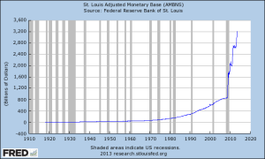
Nevertheless, the monetary base has expanded quite dramatically.
To put this in perspective, consider that the money supply has grown 370% since August 2008, just under 5 years ago. That kind of growth took nearly twenty years in the prior period (Oct 1989 to Aug 2008) and that prior period was viewed at the time to be a very high money growth period. But look at the velocity of money:
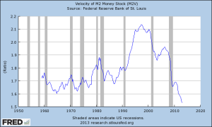
The decline is unprecedented in modern US economic history. Consider the following, as well:
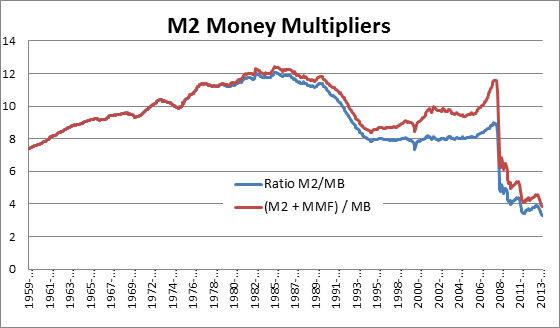
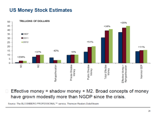
The chart shows the ratio of M2 to the monetary base (MB). The blue line is simply M2 divided by the St. Louis Adjusted Monetary Base. All data here are from FRED. Deposits became less important since the 1980’s and M3 is discontinued, therefore the red line adds institutional money market fund assets to M2 before dividing by MB. It appears to provide a more continuously sensible data series. Regardless which series one prefers, it is clear that the money multiplier is broken, at least as it relates to M2 as given. M2 is not all types of money. It includes currency, checking deposits, savings deposits, retail money market funds and small time deposits. An intuitive understanding of the money multiplier, like velocity, is how efficiently the monetary base is integrated into what people actually use to buy things. The Office of Debt Management (ODM) has termed this “effective money” and that term is a good fit as a concept. A measurement is necessary in order to use the concept. At one time, M2 was considered a reasonable assessment of effective money. That is no longer the case. In this report, ODM calculates effective money as M2 + shadow money.
This is slide 78 of the fiscal 2013 Q2 report referenced above. It is clear that no matter which measure of money that one looks at the multiplier is broken. That is, additional money has not been multiplied at all but instead been “downshifted.” This slide shows Total Effective Money has grown 34% since 2007; effective money + rehypothecation (a broader measure that this author believes is a better measure of effective money, the concept) has grown merely 20%. This is not the type of substantial money growth that Friedman had in mind when anticipating inflation.
Either the transmission mechanism is not working properly or money is being withheld from the economy or some combination of both. There are two mechanisms for money multipliers as discussed above: fractional reserve banking and collateralized banking (referred to as shadow banking). The ODM data above shows collateralized banking has collapsed by nearly half, down 42%. This is hardly surprising as private sector collateral has not grown (up 6%) and the Fed via QE has purchased and thereby withheld large portions of the public sector collateral that has grown (up 51%). In addition, the money multiplier graph above shows that the traditional fractional reserve banking relationship has also broken.
Referring to the earlier section on money creation above, the Fed has created money. That money is created as bank reserves. That is, they are on deposit with the Fed. It is an asset of the bank and the bank has the choice to exchange the cash (reserves) for another asset, such as a loan. If it does, then it needs to hold a fraction of the loan on reserve at the Fed. This is the source of the term fractional reserve banking. Reserves do not disappear; reserves are constant across the banking system but not for a particular bank. For a treatment as to why that is the case, read “Why Are Banks Holding So Many Excess Reserves” from the NY FRB. Reserves plus currency are the monetary base.
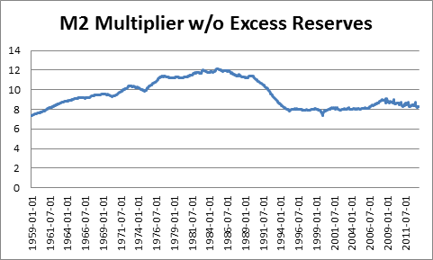
While the reserves do not disappear, they can be either required reserves backing “working” assets or excess reserves simply on deposit at the Fed. The required reserves represent money that has been multiplied. The excess reserves do not do any of the work of the economy. This chart re-draws the M2 money multiplier, but it reduces the monetary base by banks excess reserves:
Clearly, this looks far more normal. However, looking normal should not be confused with being correct. Nevertheless, the theory (that some large proportion of money is not being multiplied) and the data match. Regardless of the reason why money is being withheld as excess reserves, it is clear that so long as monetary base creation by the Fed is sitting as excess reserve balances, M2 can only grow linearly with additional money creation rather than geometrically.
Conclusion
This article has addressed monetary base creation, theoretical money multipliers and empirical money supply. At the very least, it is clear that for all of Bernanke’s effort with his helicopter, he has thus far been unable to create substantial effective money creation. Without that substantial effective money creation, money driven inflation cannot occur (a shortage of goods could still produce inflation). Until the transmission mechanism for the money multipliers kick in again, inflation will not be a problem.
The Low-Down on WTI
Paolo Santos on Seeking Alpha wrote an interesting piece titled “Weirdness Strikes the Crude Oil Market” and the current situation, on the surface, is weird. After all, according to the EIA, stockpiles of crude are essentially at the highest level in its time series. This is during a time that domestic production has dramatically increased and is expected to continue increasing. One would be forgiven for being surprised that WTI broke out of its range to higher prices. Front month WTI futures are around $103. The last time WTI traded $103 was May 2012 and that was before stockpiles went much higher than 350M barrels (they are currently close to 400M barrels). Here is a thesis to try to make sense of higher spot WTI prices amid supply.
Background
As background, the WTI-Brent spread that exploded to Brent’s favor reaching close to $25 has now collapsed below $5. Keep in mind that Brent is the inferior crude oil as it costs more to crack. Meaning, all things being equal, WTI should trade higher than Brent. All things, of course, were not equal.
Also, there was a tremendous amount of passively indexed commodity investing. Passive commodity investing is essentially always done as investment in futures and is based on three sources of return: spot price change, collateral return and roll yield. Spot price change is the change in price of the commodity itself and is what everyone is most familiar with in commodities investing. Passive investment is done using futures. One earns a collateral return on posted margin, which is usually a Treasury Bills. Most indices and funds, such as the Goldman Sachs Commodity Index (GSCI) and United States Oil ETF (USO) purchase front month futures and, near expiration, “roll” into the next month. That is, the fund sells the front month and buys the second month. If one is able to sell the front month at a higher price than the second month, then this earns a roll return. The opposite occurs if the second month is higher. When the front month is higher than the second, this is called backwardation and the reverse (2nd month higher than front month) contango. Indexed investors want backwardation to earn roll yield. As it turns out, the historical source of returns in commodities comes from the collateral and roll returns; spot price returns are volatile and average out over time (source: Expected Returns, Ilmanen).
The index and ETF investors became a very large part of the crude oil market. The impact was big enough that their futures expiration trading got its own name, the “Goldman Roll,” along with a Wikipedia page. The futures market has long since adjusted for the roll, but the point is that index investing has been a large part of the energy market for some time. That impact eventually hammered the crude oil futures market from backwardation to contango (ascribing causes in the markets can be a sketchy proposition but given the circumstances this looks like the most sensible conclusion). What is evident is that for index investors, their collateral margin was held to nearly 0% on TBills and their roll yield was now negative due to contango in the WTI market. It appears that when real yields popped from negative to positive (10 year TIP yields as proxy have move from about -.7% to .6% in 2 months – absolutely staggering), commodity investors threw in the towel and sold their underperforming funds. All three legs had negative expectations. Although I don’t have figures showing outflows from GSCI indexing, as proxy we can follow the path of USO, where outstanding shares have been on a clear, though erratic, trend down since Dec 2012. Since the beginning of 2013, shares outstanding have fallen from around 35M to 18.8M as last reported (source: Bloomberg).
The Crude Carry Trade
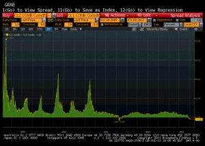
Here is a graph of the difference between the 2nd calendar WTI contract and the 1st (Bloomberg); green (positive) indicates contango and red (negative) backwardation.
Contango allows those with storage capability to buy spot crude oil to store in Cushing (the WTI delivery point) so that they could then sell the forward at a higher price earning a nice yield in the process. There is a cost to storing the oil and the rule of thumb is the cost is 45-50c per month. That coincides with the median value for the spread at 49c over the period. But the average value is 77c with a high of $8.19. One can see the volatility on the chart above. So long as things don’t look they are going to stay in backwardation, it pays to store oil and withhold it from the market. Most of the time (the median), you will break even. But on average, you can earn 27c to 32c per month due to occasional spikes. That works out to 3.6-4.3% returns in a world of ZIRP. That is far better than the passive index investor was doing and without the volatility of spot prices. In fact, it was the index investors who were assuming the volatility of the spot price and paying the carry traders to store the oil that they had purchased in the futures market.
Now WTI is in backwardation. Those in the crude carry trade need to consider the persistence of the backwardation. There has been significant withdrawal of passive investor index money. Just as passive investor demand forced crude oil into contango from backwardation, it stands to reason that flows the other way (the exit of the passive investor) would usher backwardation back. Given the evidence of investor preferences to exit passive indexing, it makes sense for the WTI carry traders to reduce their risk.
WTI-Brent Spread
The EIA released figures last week that pushed WTI higher due to a drawdown of stocks by 10M barrels. Look at those figures and note that the bulk of the drawdown is due to lower imports. Think for a moment and it makes perfect sense: traders had been diverting oil headed to other delivery points, e.g., Brent, to send to Cushing in order to satisfy end-user oil demand play the carry trade. Of course, the crude is still being produced somewhere and has to be delivered. Now that there is no carry to earn, it makes sense to send it to the Brent delivery point and make 5 extra bucks per barrel.
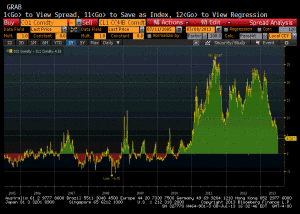
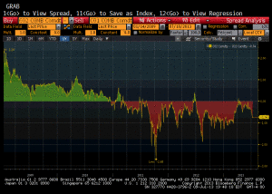
If all of that makes sense, then it stands to reason that your thinking would follow mine. And after going through this, I figured I could test the hypothesis by checking what the Brent term structure looked like over time. I expected to find that the WTI-Brent spread blow out coinciding with Brent moving into backwardation. If backwardated, Brent would no longer be a desirable place to store crude because there would be no carry trade. Here is the history of the Brent premium (Bloomberg):
And here is the same calendar spread graph (2nd – 1st ) but for Brent crude:
Note that in mid-to-late 2010 Brent moved from contango to backwardation and that was when the Brent-WTI spread began to expand. And it has stayed wide until now, when the WTI contango gave way to backwardation. Certainly it began with some fits and starts. Moving oil is not stock trading; it takes time and resources and then builds momentum. Presumably the trade gets very crowded in 2011 and becomes volatile. Nevertheless the data fits the theory. Interestingly, there were several articles in 2009 and early 2010 covering the carry trade in the Brent market.
Why then is crude staging a strong rally despite the fact that domestic US production is high and climbing plus stocks are near all-time highs? The hidden truth is that it actually is not. Brent is not making any 52 week highs and is about $1 higher than a month ago. Brent was about $120 in Feb 2013 and now is $107ish. As it turns out, that type of performance also holds for crude futures one year out. 12 Month WTI has not even traded higher than where it was in June, just a month ago. So what has happened is that 1) spot WTI is converging with Brent bringing it higher 2) there was an overall boost to the market from the drawdown and payroll figures and 3) there is general uneasiness due to news from Egypt.
Further evidence of the impact of both the carry trade and commodity index investors comes from discussions with a NY options trader. He noted that non-WTI domestic oils traded more in line with Brent than WTI. Another, a products options trader, noted that heating oil and gasoline traded closer with Brent which matches the data point that other grades of domestic oil that would be used for those products traded like the commodity (Brent), not the financial collateral (WTI). Those data points indicate that WTI is/was the aberration, not Brent. WTI, after all, is the futures market used by indexers and the market that offered the contango opportunity, not Brent and not Gulf Coast sour.
Conclusion
So the apparent weirdness that is in the crude oil market turns out to not be weird, but instead signals a shift in the crude oil marketplace. Crude and other commodities were used as collateral in financing transactions – essentially physical repo. Higher real rates, tighter money, passive investor withdrawal and backwardation have eliminated the financial motivation for withholding oil from the market. It stands to reason that WTI crude will again trade more like a commodity instead of a carry asset – at least so long as passive indexers are leaving the market.
Tactical Article on CEF Discount
Accepted by Seeking Alpha, it is here.
It discusses the current discount of CEF, a closed end fund investing exclusively in gold & silver, and its context.
Another Zoetis Article
I followed up my first article on the Zoetis deal with this one. I’m learning on the job. As I am not the most experienced at looking at deals & spinoffs, would love to hear from those that have insight.
Zoetis Article on Seeking Alpha
I recently completed a piece on why Zoetis looks like an attractive short candidate. It is a spinoff from Pfizer.
You can read the article on Seeking Alpha.

